

Regional Hydrology
Basin Characterization Model of the Great Basin: A Dataset of Historical and Future Hydrologic Response to Climate Change
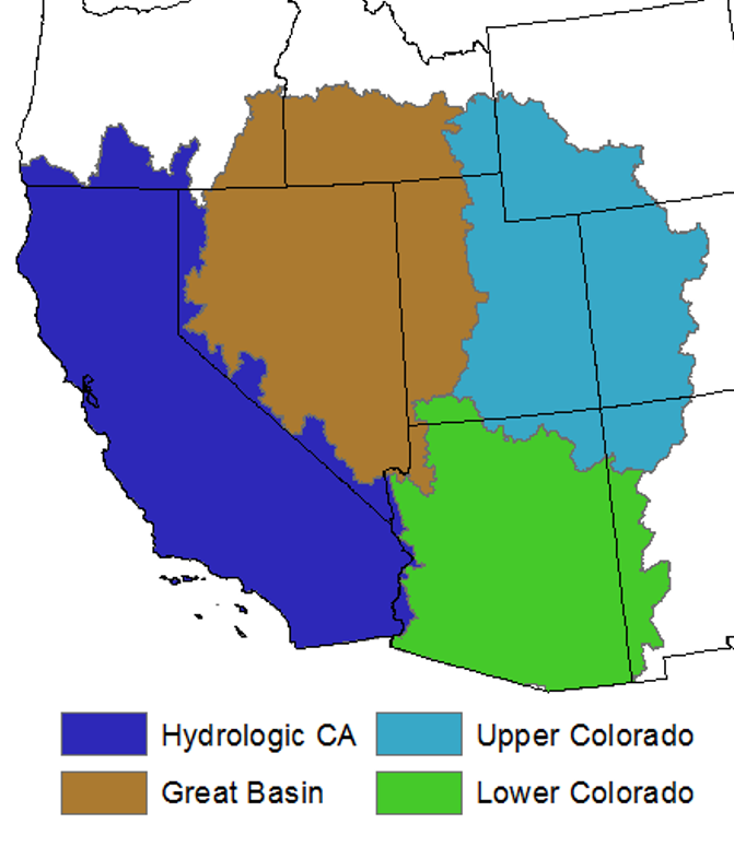
Map of the Great Basin study area in brown shown in context among completed and ongoing studies all providing consistent methods, inputs and outputs.
Ongoing changes in climate are influencing Great Basin water resources and projections of future climate scenarios are essential for assessing associated biological, physical and socioeconomic impacts. Global circulation models (GCMs) are the primary source of future climate projections. GCMs are constructed on the basis of assumed emissions scenarios or representative concentration pathways (RCPs). Because GCMs aim to capture the energy balance of the global climate system the resolution of their outputs are spatially coarse — on the order of 1-3 degrees. In addition, the archived GCM products generally include relatively simplistic variables such as minimum and maximum air temperature and precipitation at daily, monthly or annual time steps. These basic climate variables produced at coarse spatial resolutions do not offer the hydro-climatic information required by scientists, natural resource managers, conservation practitioners, and others working on climate change vulnerability assessments and adaptation planning at finer scales.
The USGS's Basin Characterization Model (BCM; Flint and others, 2013), integrates coarse climate projections with fine-scale locality data and can translate generated fine-scale maps of projected climate trends into hydrologic consequences. The BCM thus facilitates the evaluation of hydrologic response to climate change at regional, watershed, and landscape scales. This type of downscaled hydro-climatic data is essential for assessing the vulnerability of water supplies, forested and agricultural lands, biodiversity, and human health and safety.
This data release for the Great Basin BCM includes a range of downscaled climate and hydrologic response variables generated from an ensemble of climate projections within the context of the historical hydro-climatology. The Great Basin BCM (fig. 1) was developed at a 270-m spatial resolution using methods previously developed and vetted in California (Flint and Flint, 2012; Flint and others, 2013; Thorne and others 2015). Climate inputs included historical data from 1951-2013 and an ensemble of 12 future climate projections derived from the World Climate Research Programme's Coupled Model Intercomparison Project phase 5 (CMIP5) (Taylor et al, 2012). The futures were selected to provide scenarios and models that represent high rainfall and low rainfall conditions for a range of temperature increases across the entire southwest, including the completed California model plus the upper Colorado, and the lower Colorado models in progress (fig. 1). This regional approach will ensure that all the models will feature consistent futures that are ultimately contiguous across the entire region. Soils and geologic properties for the Great Basin were integrated with digital monthly maps of climate and hydrology, to generate maps representing mean annual and 30-year means for the historical (1951-1980 and 1981-2010) and future periods (2010-2039, 2040-2069, and 2070-2099).
Development of a Monthly Dataset of Historical (1951-2013), and 12 Projected Futures (2010-2099), for Climate and Hydrology for the Great Basin
The Basin Characterization Model (BCM) is a simple grid-based model that calculates the water balance for any time step or spatial scale by using the climate inputs of precipitation, minimum and maximum air temperature (Table 1). Potential evapotranspiration is calculated from solar radiation that is calculated using topographic shading and cloudiness; snow is accumulated, sublimated, and melted (sublimation, snowfall, snowpack, snowmelt); and excess water moves through the soil profile, changing the soil water storage. Changes in soil water are used to calculate actual evapotranspiration, which when subtracted from potential evapotranspiration, calculates climatic water deficit. Depending on soil properties and the permeability of underlying bedrock, water may become recharge or runoff. Routing is done via post-processing to estimate baseflow, streamflow, and groundwater recharge. The details of spatial downscaling, development of model inputs, generation of model outputs, and model calibration can be found in Flint and Flint (2012), Flint and others (2013), and Flint and Flint (2014).
| Variable | Code | Creation Method | Units | Equation/Model | Description |
|---|---|---|---|---|---|
| Maximum air temperature | tmax | Downscaled | degree C | Model input | The maximum monthly temperature, averaged annually |
| Minimum air temperature | tmin | Downscaled | degree C | Model input | The minimum monthly temperature, averaged annually |
| Precipitation | ppt | Downscaled | mm | Model input | Total monthly precipitation (rain or snow), summed annually |
| Potential evapotranspiration | pet | Modeled/pre-processing input for BCM | mm | Model input; modeled on an hourly basis from solar radiation that is modeled using topographic shading, corrected for cloudiness, and partitioned on the basis of vegetation cover to represent bare-soil evaporation and evapotranspiration due to vegetation | Total amount of water that can evaporate from the ground surface or be transpired by plants, summed annually |
| Runoff | run | BCM | mm | Model output; amount of water that exceeds total soil storage + rejected recharge | Amount of water that becomes streamflow, summed annually |
| Recharge | rch | BCM | mm | Model output; amount of water exceeding field capacity that enters bedrock, occurs at a rate determined by the hydraulic conductivity of the underlying materials, excess water (rejected recharge) is added to runoff | Amount of water that penetrates below the root zone, summed annually |
| Climatic water deficit | cwd | BCM | mm | Model output; pet-aet | Annual evaporated demand that exceeds available water, summed annually |
| Actual evapotranspiration | aet | BCM | mm | Model output; pet calculated when soil water content is above wilting point | Amount of water that evaporates from the surface and is transpired by plants if the total amount of water is not limited, summed annually |
| Sublimation | subl | BCM | mm | Model output; calculated, applied to pck | Amount of snow lost to sublimation (snow to water vapor), summed annually |
| Soil water storage | stor | BCM | mm | Model output; ppt + melt - aet - rch - run | Average amount of water stored in the soil annually |
| Snowfall | snow | BCM | mm | Model output; precipitation if air temperature below 1.5 degrees C (calibrated) | Amount of snow that fell, summed annually |
| Snowpack | pck | BCM | mm | Model output; prior month pck + snow - subl - melt | Amount of snow that accumulated per month, summed annually (if divided by 12 would be average monthly snowpack) |
| Snowmelt | melt | BCM | mm | Model output; calculated, applied to pck | Amount of snow that melted, summed annually (snow to liquid water) |
| Excess water | exc | BCM | mm | Model output; ppt - pet | Amount of snow that melted, summed annually (snow to liquid water) |
Table 1. Input climate and output hydrology variables for the Basin Characterization Model, with codes used in filenames, and description of calculations (from Thorne and others, 2012). [C, celsius; mm, millimeter; BCM, Basin Characterization Model.)
Calibration of the Great Basin BCM to measured streamflow followed methods described in Flint and others (2013). A subset of 44 basins, with relatively unimpaired streamflow (Fig. 2a), was selected from the USGS GAGES II dataset (Falcone, 2011). Calibration results are in Table 2, which provides gage IDs, basin areas, calibration parameters, and goodness-of-fit statistics.
| Calibration Parameters | Goodness-of-Fit Statistics | |||||||
|---|---|---|---|---|---|---|---|---|
| Station ID | Basin Name | Basin Area (km2) | SurfaceExp | ShallowExp | DeepExp | AquiferRch | r2 | NSS |
| 09404222 | Spencer Crk nr Peach Springs, AZ | 647 | 0.7 | 0.6 | 1.6 | 0.72 | 0.58 | |
| 09413900 | Beaver Dam Wash nr Enterprise, UT | 148 | 0.6 | 0.5 | 0.97 | 0.40 | 0.38 | |
| 09415460 | White Riv nr Red Mtn nr Preston, NV | 73 | 0.85 | 0.7 | 1 | 0.75 | 0.71 | |
| 09415515 | Water Canyon Crk nr Preston, NV | 28 | 0.85 | 0.6 | 0.44 | 0.27 | -1.17 | |
| 09417500 | Meadow Valley Wash at Eagle Cyn nr Ursine, NV | 748 | 0.99 | 0.9 | 0.15 | 0.35 | 0.32 | |
| 09419610 | Lee Canyon nr Charleston Park, NV | 24 | 0.9 | 0.6 | 0.042 | 1.00 | 0.90 | |
| 10172700 | Vernon Creek nr Vernon, UT | 69 | 0.99 | 0.9 | 0.35 | 0.47 | 0.45 | |
| 10172800 | South Willow Creek nr Grantsville, UT | 11 | 0.75 | 0.75 | 1.35 | 0.83 | 0.83 | |
| 10172870 | Trout Creek nr Callao, UT | 21 | 0.7 | 0.75 | 0.98 | 0.85 | 0.81 | |
| 10224100 | Oak Creek abv Little Creek nr Oak City, UT | 15 | 0.7 | 0.7 | 0.99 | 0.74 | 0.74 | |
| 10234500 | Beaver River nr Beaver, UT | 235 | 0.7 | 0.8 | 0.86 | 0.88 | 0.85 | |
| 10242000 | Coal Creek nr Cedar City, UT | 206 | 0.75 | 0.8 | 1 | 0.69 | 0.29 | |
| 10243260 | Lehman Creek nr Baker, NV | 28 | 0.8 | 0.8 | 0.75 | 0.70 | 0.58 | |
| 10243700 | Cleve Creek nr Ely, NV | 82 | 0.75 | 0.7 | 0.68 | 0.64 | 0.59 | |
| 10244950 | Steptoe Creek nr Ely, NV | 29 | 0.97 | 0.8 | 1 | 0.63 | 0.55 | |
| 10245445 | Illipah Creek nr Hamilton, NV | 80 | 0.7 | 0.8 | 0.6 | 0.64 | 0.42 | |
| 10245900 | Pine Creek nr Belmont, NV | 31 | 0.5 | 0.8 | 0.6 | 0.61 | 0.45 | |
| 10245910 | Mosquito Creek nr Belmont, NV | 39 | 0.8 | 0.7 | 0.2 | 0.47 | -0.09 | |
| 10246846 | L Currant Creek nr Currant, NV | 34 | 0.45 | 0.4 | 1.8 | 0.63 | 0.59 | |
| 10249280 | Kingston Creek blw Cougar Cyn nr Austin, NV | 60 | 0.75 | 0.75 | 0.6 | 0.73 | 0.74 | |
| 10249300 | Twin River nr Round Mountain, NV | 50 | 0.75 | 0.75 | 0.6 | 0.69 | 0.68 | |
| 10313400 | Mary's River blw Orange Brg nr Charleston, NV | 183 | 0.98 | 0.8 | 1 | 0.56 | 0.36 | |
| 10316500 | Lamoille Creek nr Lamoille, NV | 65 | 0.88 | 0.2 | 1.85 | 0.89 | 0.89 | |
| 10317500 | N Fk Humboldt River at Devils Gate nr Halleck, NV | 2261 | 0.97 | 0.69 | 0.46 | 0.55 | 0.52 | |
| 10321590 | Susie Creek at Carlin, NV | 476.1680.99 | 0.97 | 0.6 | 0.5 | 0.41 | 0.33 | |
| 10321950 | Maggie Creek at Maggie Creek Cyn nr Carlin, NV | 892.7970.99 | 0.98 | 0.5 | 0.85 | 0.22 | -0.16 | |
| 10329500 | Martin Creek nr Paradise Valley, NV | 454.520.98 | 0.75 | 0.68 | 0.5 | 0.55 | 0.51 | |
| 10353000 | Kings River nr Orovada, NV | 52.22250.99 | 0.5 | 0.8 | 0.5 | 0.63 | 0.62 | |
| 13161500 | Bruneau River at Rowland, NV | 986.130.98 | 0.7 | 0.8 | 0.95 | 0.68 | 0.67 | |
| 13162225 | Jarbridge River blw Jarbridge, NV | 76.13370.99 | 0.9 | 0.7 | 0.92 | 0.73 | 0.71 | |
| 13169500 | Big Jacks Creek nr Bruneau, ID | 631.6270.98 | 0.9 | 0.6 | 0.22 | 0.29 | -0.11 | |
| 13185000 | Boise River nr Twin Springs, ID | 2154.390.98 | 0.85 | 0.7 | 1 | 0.78 | 0.75 | |
Table 2. Table 2. Streamgages and basins used in model calibration for the Great Basin, including calibration coefficients and goodness-of-fit statistics. [km2, square kilometers; r2, coefficient of determination; NSS, Nash-Sutcliffe efficiency statistic]
Input and output data for the Great Basin BCM are included as available data in this data release: gridded monthly climate data (Daly and others, 2008; Taylor and others, 2012); geology (Jennings 1977); soil water content (field capacity and wilting point) and soil porosity calculated from texture (percent sand, silt, and clay) and organic matter and soil depth, available from the SSURGO soil database (NRCS, 2006). Calculated soil storage (field capacity minus wilting point multiplied by depth) is shown in Figure 2a, and geology in Figure 2b, providing the level of detail of input data that the model uses, and the range of geologic types in the study area. Also included in this dataset are annual values for each water year (October 1 to September 30) for precipitation, minimum and maximum air temperature, potential evapotranspiration, actual evapotranspiration, climatic water deficit (potential minus actual evapotranspiration, corresponding to landscape stress and demand), runoff and recharge, and April 1st snowpack. Statistics calculated for 30-year periods (1951-1980 and 1981-2010) and futures (2010-2039, 2040-2069, and 2070-2099) include mean, detrended standard deviation, and standard deviation, mean winter air temperature (December, January, February; DJF), and mean summer air temperature (June, July, August; JJA).
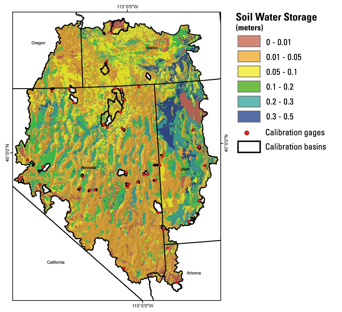
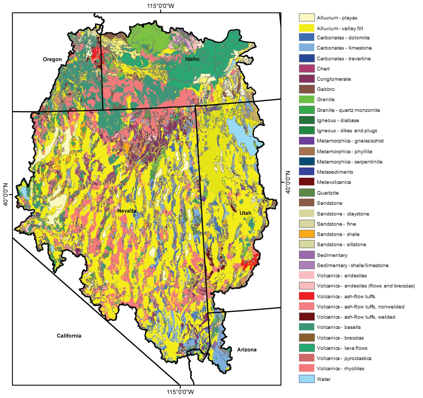
Maps of input properties for (A) soil storage and (B) geologic type used in the Basin Characterization Model for the Great Basin.
Model Selection for Great Basin Climate Projections
We selected an ensemble of future climate projections (Table 3) from the World Climate Research Programme's Coupled Model Intercomparison Project phase 5 (CMIP5). CMIP5 data for the continental US (Taylor et al, 2012) were downscaled to 12-km using the Bias Corrected Statistically Downscaled (BCSD) (Wood et al., 2004) methodology. These projections align with those adopted in the Intergovernmental Panel on Climate Change 5th assessment report (AR5; IPCC, 2014). The AR5 projections include representative concentration pathways (RCPs) that describe four potential 21st century pathways of greenhouse gas emissions and resultant atmospheric concentrations as well as air pollutant emissions and land-use changes. The RCPs include a stringent mitigation scenario (RCP2.6) that aims to constrain global warming at or below 2°C greater than pre-industrial air temperatures. There are two intermediate scenarios (RCP4.5 and RCP6.0) and one scenario with high greenhouse gas emissions (RCP8.5). RCP6.0 and RCP8.5 scenarios model conditions resulting from failure to adopt stringent efforts to constrain emissions.
| Originating Group(s) | Country | Model Abbreviation | Representative Concentration Pathway |
|---|---|---|---|
| Commonwealth Scientific and Industrial Research Organization (*CSIRO) and Bureau of Meteorology (BOM) | Australia | ACCESS1_0 | 4.5, 8.5 |
| Canadian Centre for Climate Modelling and Analysis | Canada | CANESM2 | 2.6, 4.5, 8.5 |
| National Center for Atmospheric Research | USA | CCSM4 | 2.6, 4.5, 6.0, 8.5 |
| Community Earth System Model Contributors | USA | CESM1_BGC | 4.5, 8.5 |
| Centro Euro-Mediterraneo per I Cambiamenti Climatici | Europe | CMCC_CM | 4.5, 8.5 |
| Centre National de Recherches Météorologiques / Centre Européen de Recherche et Formation Avancée en Calcul Scientifique | France | CNRM-CM5 | 4.5, 8.5 |
| LASG, Institute of Atmospheric Physics, Chinese Academy of Sciences and CESS,Tsinghua University | China | FGOALS-G2 | 2.6, 4.5, 8.5 |
| US Dept. of Commerce / NOAA / Geophysical Fluid Dynamics Laboratory | USA | GFDL_CM3 | 2.6, 4.5, 6.0, 8.5 |
| US Dept. of Commerce / NOAA / Geophysical Fluid Dynamics Laboratory | USA | GFDL_ESM2M | 2.6, 4.5, 6.0, 8.5 |
| NASA / Goddard Institute for Space Studies | USA | GISS_ER_R | 2.6, 4.5, 6.0, 8.5 |
| Hadley Centre for Climate Prediction and Research / Met Office | UK | HADGEM2_CC | 4.5, 8.5 |
| Hadley Centre for Climate Prediction and Research / Met Office | UK | HADGEM2_ES | 2.6, 4.5, 6.0, 8.5 |
| Institut Pierre Simon Laplace | France | IPSL-CM5A-LR | 2.6, 4.5, 6.0, 8.5 |
| Center for Climate System Research (The University of Tokyo), National Institute for Environmental Studies, and Frontier Research Center for Global Change (JAMSTEC) | Japan | MIROC-ESM | 2.6, 4.5, 6.0, 8.5 |
| Center for Climate System Research (The University of Tokyo), National Institute for Environmental Studies, and Frontier Research Center for Global Change (JAMSTEC) | Japan | MIROC5 | 2.6, 4.5, 6.0, 8.5 |
| Max-Planck-Institut für Meteorologie (Max Planck Institute for Meteorology) | Germany | MPI-ESM-LR | 2.6, 4.5, 8.5 |
| Meteorological Research Institute | Japan | MRI-CGCM3 | 2.6, 4.5, 8.5 |
Table 3. Global climate models considered in the selection process for input to the Basin Characterization Model of the Great Basin. Note that all models include representative concentration pathways (RCP) 4.5 and 8.5, but RCP2.6 and RCP6.0 are only available for a subset of models.
A subset of the CMIP5 climate futures, defined as a combination of a GCM and a representative concentration pathway emissions scenario, listed in Table 3 was selected using a statistical cluster analysis to represent the full range of potential climate projections, from warm and wet to hot and dry (details below). These climate futures were then further downscaled to 270 m and used as input into the BCM to generate a suite of climate and hydrologic response variables that have direct relevance for conservation and management of the Great Basin's natural resources and adaptation strategies. We chose to select futures to provide scenarios and models that represented wet and dry conditions for a range of temperature increases across the entire southwest, including the completed California model, and the upper Colorado, and the lower Colorado, both of which are in progress (fig. 1). As a result, all the models, once completed, will reflect consistent methodologies and applied futures to generate a contiguous set of results across the entire region. We are therefore including all 4 model domains in the methods description for model selection.
We did not select a "most likely" future climate trajectory; such a goal is fundamentally impossible given the uncertainties in emissions, model performance, and the inherent unpredictability of short-term climatic variability. The goal of having a wide-ranging ensemble of climate futures is to "expose" particular hydrological and ecological systems to varying degrees of climate change, quantify their modeled responses, and understand when and where the limits of acceptable system performance are exceeded in a "scenario-neutral" approach (Prudhomme and others, 2010; Brown, 2012). Given the known climate sensitivities of arid, semi-arid, and seasonally dry landscapes in the Great Basin this approach permits a sensitivity analysis of the landscape that can identify areas or watersheds that will be most impacted, and those that may be least affected across a range of climate projections.
A cluster analysis used effectively reduced the number of futures needed to capture the full range of variability among CMIP5 futures. Seasonal and maximum annual air temperature (Tmax), minimum annual air temperature (Tmin), and annual and seasonal precipitation (PPT) were averaged into three 30-year periods (2010-2039, 2040-2069, and 2070-2099). The 30-year periods were defined as climate "normals," consistent with standard climatology. Seasonal summaries included fall (September-October-November, SON), winter (December-January-February, DJF), spring (March-April-May, MAM) and summer (June-July-August, JJA).
Spatial averages of these seasonal and annual 30-year averages of Tmax and PPT were calculated for four regions: California, Great Basin, Upper Colorado, and Lower Colorado. The cluster analysis used only end of-century climate (2070-2099). All of the annual and seasonal temperature variables were highly correlated (r>0.9) which justified using only annual Tmax in the cluster analysis. Seasonal PPT was used to identify the relative inputs of winter Pacific storms and summer monsoonal moisture. Some of the remaining variability among Tmin and Tmax at the seasonal scale is associated with varying precipitation, so screening on PPT captures this aspect of variability. For example, there is generally a positive correlation between seasonal Tmin and precipitation, reflecting warmer nights under cloudy conditions. The cluster analysis to group climate futures was completed (JMP 10.0, SAS Institute), using Wards agglomerative method. The number of clusters chosen was based on the inflection point of cumulative variance explained.
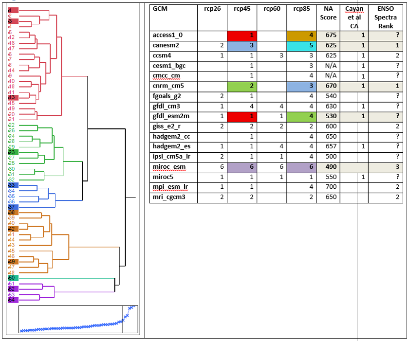
Figure 3. Results of cluster analysis, including dendrogram on left, cumulative variance plot, bottom left with selection point noted, model selection, North American (NA) skill scores, 4th assessment models (Cayan et al. CA), and ENSO spectra rank.
The cluster diagram indicated as a dendrogram on the left shows a 6 cluster solution, with cluster size ranging from 1 to 21 futures. Clusters are color-coded. The 6 cluster choice corresponds to the inflection point in the cumulative variance plot below the dendrogram, and suggests that 6 clusters are sufficient to capture ~ 50% of the variability and that additional clusters have a low marginal value. At least one future from each cluster is necessary to capture the range of variability. The final choices were informed by other criteria, such as consistency in emissions scenario referred to as representative concentration pathways (RCP), model performance, expert opinions, and use by other climate change assessments.
The identities of the futures by cluster is shown on the right, along with some ancillary information such as North American (NA) skill (Watterson and others, 2014), choice by experts in CA for California's 4th climate assessment (Pierce and others, 2015), and ENSO spectra rank. The final set of 12 futures is highlighted by cluster color. The set is necessarily a compromise. Where possible, futures considered by Pierce and others (2015) for California were chosen, to allow for comparability across larger spatial domains. The two wetter models (CanESM2 and CNRM_CM5) both had high NA skill. While MirocESM had poorer NA skill, the distinctive response and segregation into its own cluster merited its inclusion in the ensemble. MirocESM was the driest model overall, especially the RCP8.5 run, and represents an extreme scenario worth investigating for adaptation limits.
We plot Tmax and PPT for three 30-year normals in the original 54 futures (Figure 4), and the 12 selected futures are highlighted in black. The selected futures span the full range of PPT and Tmax projected by all 54 futures over the next century. The climatological differences among the regions are clearly seen.
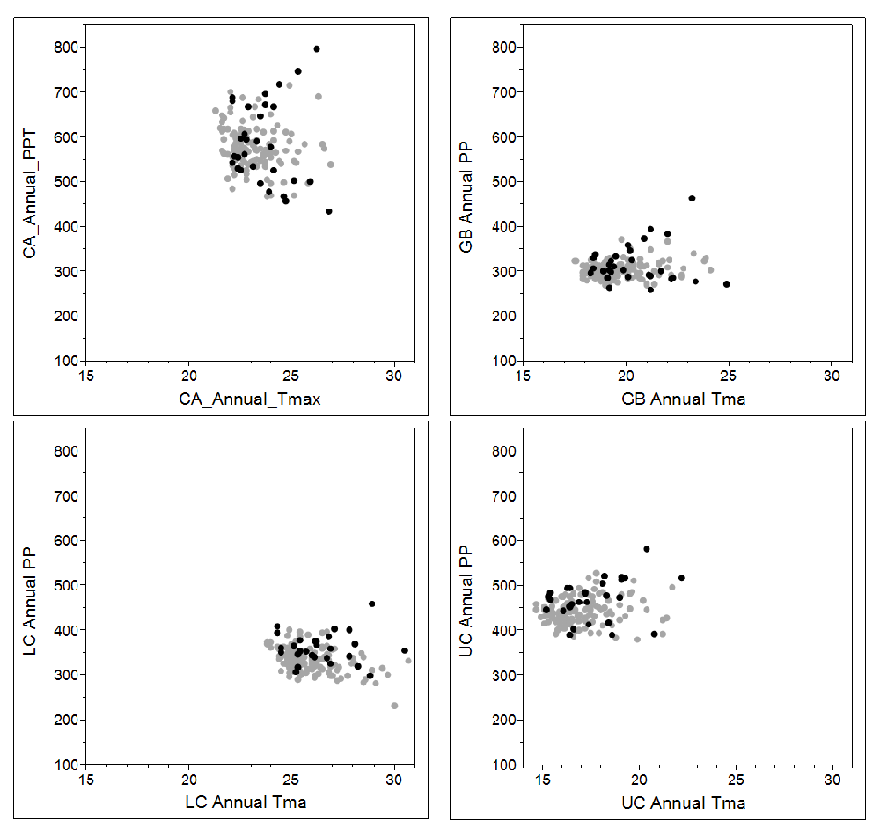
Figure 4. 30-year average annual values for annual maximum air temperature (Tmax) and precipitation (PPT) for each region, all periods. Black circles are selected ensemble members, grey are the remainder. CA is California, GB is Great Basin, LC is Lower Colorado, and UC is Upper Colorado.
The summer monsoon (represented by JJA PPT) in the Great Basin is a critical climatological feature that was reproduced in the selected futures (Figure 5). Most futures remain within a range of 40-55 mm, close to the historical average. We did not detect large projected trends with the exception of Canesm2, which greatly increases JJA precipitation, especially in rcp85. ACCESS1_0-rcp45 projects the driest monsoon seasons, less than 40 mm.
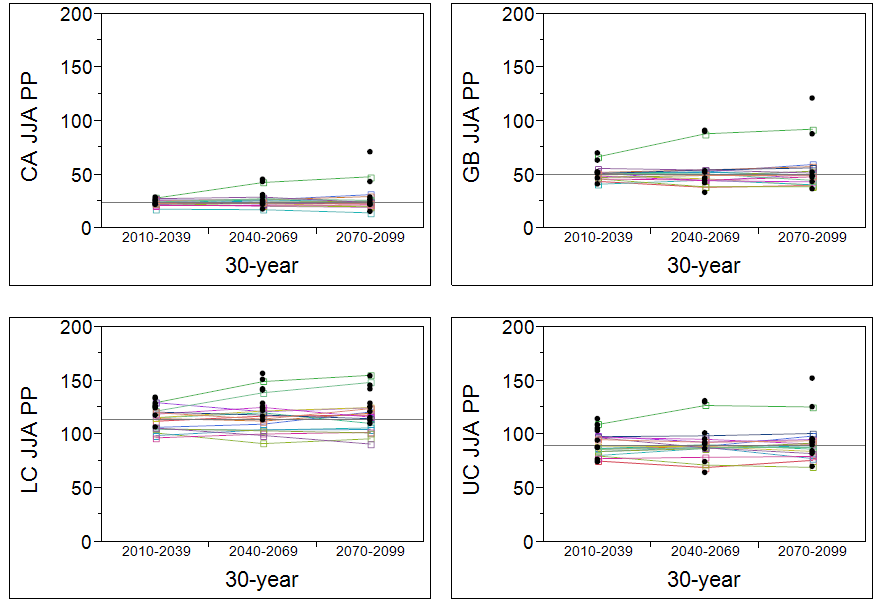
Figure 5. Thirty-year means of monsoon (summer; JJA) rainfall for all models for all model domains. Lines connect model means for RCP45 and RCP85. Historical mean is the horizontal line.
Monthly Climate and Hydrology for Historical (1951-2013), and 12 Projected Futures (2011-2099), for the Great Basin Region
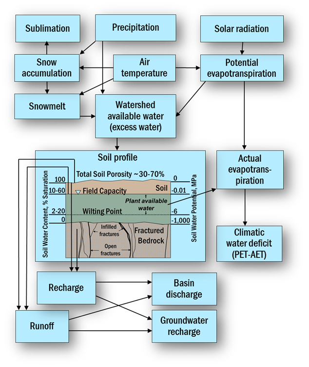
Figure 2. Schematic describing relation of components of the Basin Characterization Model (from Thorne and others, 2012).
The Basin Characterization Model (BCM) is a simple grid-based model that calculates the water balance for any time step or spatial scale by using climate inputs, precipitation, minimum and maximum air temperature. Potential evapotranspiration is calculated from solar radiation with topographic shading and cloudiness, snow is accumulated, sublimated, and melted (sublimation, snowfall, snowpack, snowmelt), and excess water moves through the soil profile, changing the soil water storage. Changes in soil water are used to calculate actual evapotranspiration, and when subtracted from potential evapotranspiration calculates climatic water deficit. Depending on soil properties and the permeability of underlying bedrock, water may become recharge or runoff. Routing is done via post-processing to estimate baseflow, streamflow, and groundwater recharge (see Flint and others, 2013). Monthly downscaled climate inputs and hydrologic output variables (Table 1) can be examined for any size polygon representing regions or watersheds, or the distribution across the landscape.
Detailed schematics, inputs and outputs can be found at https://ca.water.usgs.gov/projects/reg_hydro/projects/dataset.html. All methods and datasets follow those described in Flint and others (2013) with the exception of revised soil properties. Revisions were made to increase the soil water holding capacity to improve matches of BCM recharge estimates for the Great Basin to local estimates of recharge and measured data.
The BCM uses soil data sets from both the Soil Survey Geographical Database (SSURGO) and State Soil Geographic Database (STATSGO) (Miller and White, 1998; Wieczorek, 2013; Wieczorek, 2014). STATSGO is a coarse national dataset and is only used to fill in gaps that exist in the finer resolution SSURGO dataset. The data needed for the BCM are soil depth, soil porosity, and water content at field capacity and wilting point. Available water capacity is the water content at field capacity minus the water content at wilting point times the soil depth. Both SSURGO and STATSGO provide water content at field capacity as water content at a matric potential of -0.33 bars (-0.033MPa) and wilting point as water content at a matric potential of -15.0 bars (-1.5MPa). Although these numbers have been used to date by the BCM, current research has shown that the BCM has a tendency to overestimate recharge (RCH) by under estimating actual evapotranspiration (AET). Several methods were evaluated to develop better estimates of RCH and AET. Both SSURGO and STATSGO limit soil depth to 2.01 m, however plant rooting depths can penetrate below this arbitrary maximum soil depth and extract additional water thus increasing AET and reducing RCH. Adding additional soil depth helped in some cases, however in many cases increasing soil depth by 10 m was not deep enough to match AET or RCH where we had good estimates of both. In these cases water content at field capacity and wilting point were within a couple of percent of each other so even with the additional depth the soil could not hold enough water to match AET. Many plants, especially desert plants, can remove water to wilting points of <-60 bars (-6.0 MPa) and many natural field soils (non-agricultural) have field capacities more on the order of -0.10 bars (-0.01 MPa) (Flint and Childs, 1984a,b). Changing field capacity and wilting point to water content at these water potentials can increase the water holding capacity in most locations.
In order to develop a range of water contents at different matric potentials using soil texture and organic matter from SSURGO and STATSGO, a variety of soil physics based equations were investigated (Campbell, 1985; Gupta and Larson, 1979; Rawls, and others, 2003; Saxton and Rawls, 2006). These equations, often based on the same laboratory data sets, are in general agreement with each other but some provide more utility than others. Organic matter is an important contributor to available water capacity (Gupta and Larson, 1979; Hudson, 1994; Huntington, 2006; Rawls and others, 2003; Saxton and Rawls, 2006). Saxton and Rawls (2006) incorporated the relation between organic matter and available water capacity and provided enough information that we could develop water retention equations for each soil type using a simple power function (Brooks and Corey, 1964). These new equations were used with soil texture (percent sand, silt, and clay) and percent organic matter to develop water retention curves for each location and we used water content at -0.1 bars for field capacity and -30 bars for wilting point to run the BCM for the Great Basin.
Monthly Climate and Hydrology for Historical (1951-2013), and 12 Projected Futures (2011-2099), for the Great Basin Region
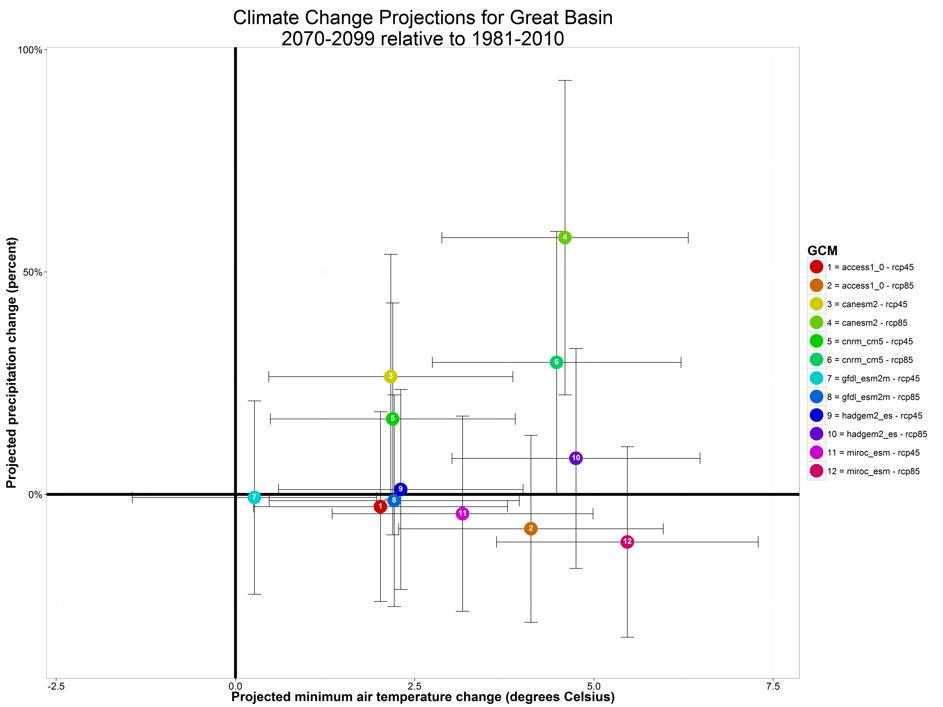
Figure 6. Projected change in precipitation and minimum air temperature for 30-year water year means between 1951-1980 and 2070-2099 for12 future climate projections. Bars indicate the range of values for all cells in the Great Basin and boxes indicate general direction of precipitation and temperature change in comparison to the ensemble mean.
Climate and hydrologic response variables are available for both historical and future climate projections at a 270-m grid-scale. Data are available via web-based download for the Great Basin hydrologic region or selected subsets. The 12 climate change projections (Table 2) span a range of potential future climates, with all air temperature projections higher by the end of the 21st century, and variable changes in precipitation (Figure 6).
Thirty-year means, standard deviation, and detrended standard deviation for all climate and hydrologic variables (ppt, tmin, tmax, pet, aet, cwd, Apr 1 snowpack, rch, run) as well as 30-year means of these variables for each month are available from California Climate Commons for historical and future time periods, and all monthly data is available from the USGS Geo Data Portal (availability pending). Thirty-year periods are 1951-1980, 1981-2010, 2010-2039, 2040-2069, and 2070-2099.
Examples of output are shown in the following maps illustrating future precipitation in comparison to current for a wet and dry scenario (Figure 7), future CWD in comparison to current for a wet and dry scenario (Figure 8), historical distribution of recharge, and future recharge in comparison to historical for a wet model and a dry model (Figure 10).
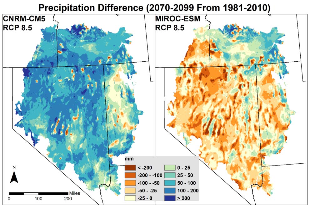
Figure 7. Future (2070-2099) precipitation in comparison to historical (1981-2010) for a wet model (CNRM-CM5) and a dry model (MIROC-ESM) both for business-as-usual scenario rcp 8.5.
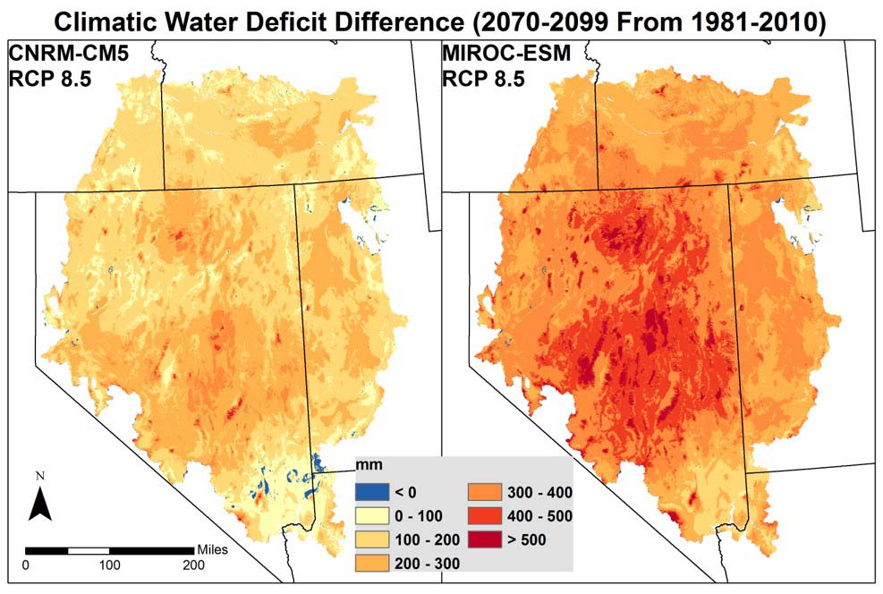
Figure 8. Future (2070-2099) climatic water deficit in comparison to historical (1981-2010) for a wet model (CNRM-CM5) and a dry model (MIROC-ESM) both for business-as-usual scenario rcp 8.5.
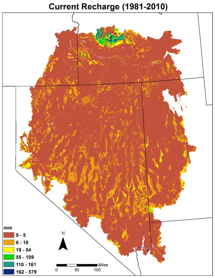
Figure 9. Historical (1981-2010) distribution of recharge.
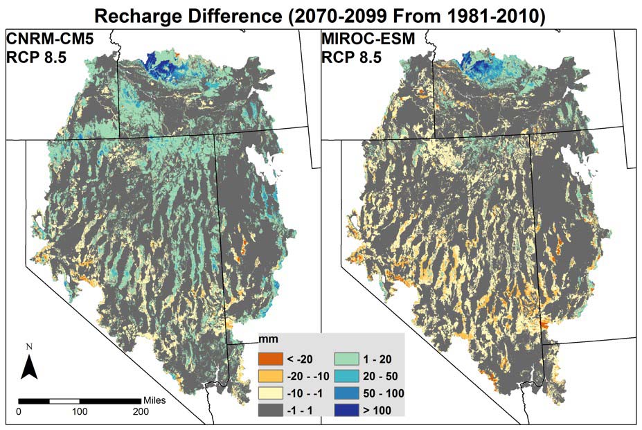
Figure 10. Future (2070-2099) recharge in comparison to historical (1981-2010) for a wet model (CNRM-CM5) and a dry model (MIROC-ESM) both for business-as-usual scenario rcp 8.5.
References
Bhaskar J., Z.Z. Hu, and A. Kumar. 2013. SST and ENSO variability and change simulated in historical experiments of CMIP5 models. Climate Dynamics DOI 10.1007/s00382-013-1803-z
Brooks, R.H. and Corey, A.T.: "Hydraulic properties of porous media," Hydraulic paper no. 3, Colorado State University, 1964
Brown, C. and R.L. Wilby. 2012. An alternate approach to assessing climate risks. Eos 92(41):401-402.
Campbell, G.S., 1985. Soil physics with basic, transport models for soil-plant systems, Elsevier, New York, 150pp.
Daly, C., Halbleib, M., Smith, J.I., Gibson, W.P., Doggett, M.K., Taylor, G.H., Curtis, B.J., Pasteris, P.P., 2008, Physiographically sensitive mapping of climatological temperature and precipitation across the conterminous United States: Int J Climatol 28:2031-2064.
Falcone, J.A., 2011, GAGES–II, Geospatial Attributes of Gages for Evaluating Streamflow [digital spatial dataset], available at https://water.usgs.gov/GIS/metadata/usgswrd/XML/gagesII_Sept2011.xml.
Flint, A. L. and Childs, S. W., 1984a, Measuring soil water availability in the field: Oregon State University Extension Service, Forestry Intensified Research Report, 6(2): 6 7. Medford, OR.
Flint, A. L. and Childs, S. W., 1984b, Physical properties of rock fragments and their effect on available water in skeletal soils: Soil Science Society America Special Publication #13: Erosion and Productivity of Soils Containing Rock Fragments, June 1984, pp. 91 103.
Flint, L.E., Flint, A.L., 2012, Downscaling future climate scenarios to fine scales for hydrologic and ecological modeling and analysis: Ecological Processes 2012 1:1. doi:10.1186/2192-1709-1-2
Flint, L.E. and Flint, A.L., 2014, California Basin Characterization Model: A Dataset of Historical and Future Hydrologic Response to Climate Change, U.S. Geological Survey Data Release, doi:10.5066/F76T0JPB
Flint, L.E., Flint, A.L., Thorne, J.H., and Boynton, R., 2013, Fine-scale hydrologic modeling for regional landscape applications: the California Basin Characterization Model development and performance: Ecol. Processes 2:25.
Gupta, S.C. and Larson, W.E., 1979, Estimating soil water retention characteristics from particle size distribution, organic matter percent, and bulk density, Water Resources Research Vol. 15, No.6.
Hudson, B. 1994. Soil organic matter and available water capacity, J. Soil Water Conserv. 49:189-193.
Huntington, T.G., 2006, Available water capacity and soil organic matter, In Encyclopedia of Soil Science, Second Edition. Taylor and Francis: New York, Published online: 12 Dec 2007: 139-143. DOI: 10.1081/E-ESS-120018496.
IPCC, 2007, IPCC Fourth Assessment Report: Climate change 2007; synthesis report. Core writing team, Pachauri, R. K. and Reisinger A. (Eds). International Panel on Climate Change, Geneva Switzerland.
Jennings, C.W., 1977, Geologic map of California. California Division of Mines and Geology geologic data: Map number 2, scale 1:750,000.
Miller, D.A. and R.A. White, 1998: A Conterminous United States Multi-Layer Soil Characteristics Data Set for Regional Climate and Hydrology Modeling. Earth Interactions, 2. doi: http://dx.doi.org/10.1175/1087-3562(1998)002<0001:ACUSMS>2.3.CO;2. Accessed [July 23, 2015).
NRCS (Natural Resources Conservation Service), 2006, U.S. General Soil Map (SSURGO/STATSGO2): Data, Description
Prudhomme, C., R.L. Wilby, S. Crooks, A.L. Kay, and N.S. Reynard. 2010. Scenario-neutral approach to climate change impact studies: application to flood risk. J. Hydrol. 390:198–209.
Rawls, W.J., Pachepsky, Y.A., Ritchie, J.C., Sobecki, T.M., and Bloodworth, 2003, Effect of soil organic carbon on soil water retention, Geoderma, 116, pp61-76.
Saxton, K.E. and Rawls, W.J., 2006, Soil water characteristic by texture and organic matter for hydrologic solutions, Soil Sci. Soc. Am. J. 70:1569-1578.
Taylor, K.E., R.J. Stouffer, G.A. Meehl: An Overview of CMIP5 and the experiment design. Bull. Amer. Meteor. Soc., 93, 485-498, doi:10.1175/BAMS-D-11-00094.1
Thorne, J.H., Boynton, R., Flint, L.E., Flint, A.L., Le, T.N., 2012, Development and application of downscaled hydroclimatic predictor variables for use in climate vulnerability and assessment studies: CEC-500-2012-010. California Energy Commission, Sacramento.
Watterson, I.G., J. Bathols, and C. Heady. 2014. What influences the skill of climate models over the continents? Bulletin of the American Meteorological Society May 2014:690-700 DOI:10.1175/BAMS-D-12-00136.1
Wieczorek, M.E., 2014. Area- and Depth-Weighted Averages of Selected SSURGO Variables for the Conterminous United States and District of Columbia. USGS Data Series 866. Available on-line at http://water.usgs.gov/lookup/getspatial?ds866_ssurgo_variables. Accessed [July 23, 2015).
Wieczorek, M.E., 2015. STATSGO2 Area- and Depth- Weighted Averages of Selected STATSGO2 Variables. Science Base-Catalog. Available on-line at https://www.sciencebase.gov/catalog/item/54b97608e4b043905e00fc9d. Accessed [July 23, 2015).
Wood, A.W., Leung, L.R., Sridhar, V., and Lettenmaier, D.P., 2004, Hydrologic implications of dynamical and statistical approaches to downscaling climate model outputs: Climatic Change, 62, 189-216.
Publications
Basin Characterization Model Development
Flint, L.E. and Flint, A.L., 2014, California Basin Characterization Model: A Dataset of Historical and Future Hydrologic Response to Climate Change, U.S. Geological Survey Data Release, doi:10.5066/F76T0JPB
Flint, L.E., Flint, A.L., and Thorne, J.H., 2014, Evaluating Climate Change Using the Basin Characterization Model: USGS Fact Sheet 2014-3098
Flint, L.E., Flint, A.L., Thorne, J.H., and Boynton, R., 2013, Fine-scale hydrological modeling for climate change applications; using watershed calibrations to assess model performance for landscape projections; Ecological Processes 2:25
Thorne, J.H., Boynton, R., Flint, L.E., Flint, A.L., and Le, T-N., 2012, Development and application of downscaled hydroclimatic predictor variables for use in climate vulnerability and assessment studies. California Energy Commission. Publication number: CEC-500-2012-010.
Flint, L.E., Flint, A.L., 2012, Downscaling future climate scenarios to fine scales for hydrologic and ecological modeling and analysis: Ecological Processes 2012 1:1. doi:10.1186/2192-1709-1-2
Flint, L.E., and Flint, A.L., 2012, Estimation of Stream Temperature in Support of Fish Production Modeling under Future Climates in the Klamath River Basin: USGS Scientific Investigations Report 2011-5171, vi, 31 p.
Flint, L.E., and Flint, A.L., 2008, Regional analysis of ground-water recharge, in Stonestrom, D.A., Constantz, J., Ferré, T.P.A., and Leake, S.A., eds., Ground-water recharge in the arid and semiarid southwestern United States: U.S. Geological Survey Professional Paper 1703, p. 29-59.
Flint, A.L., and Flint, L.E., 2008, Integration of regional hydrologic modeling using FORTRAN and ArcGIS, Water Resources IMPACT 10(1) p. 31-35.
Flint, A.L., Flint, L.E., Hevesi, J.A., and Blainey, J.M., 2004, Fundamental concepts of recharge in the Desert Southwest: a regional modeling perspective, in Groundwater Recharge in a Desert Environment: The Southwestern United States, edited by J.F. Hogan, F.M. Phillips, and B.R. Scanlon, Water Science and Applications Series, vol. 9, AGU, Washington, D.C., 159-184.
Flint, A.L., 2004, Recharge mapping at Yucca Mountain, Nevada — the scale effect; Box 4-2 in Groundwater Fluxes Across Interfaces, National Research Council, National Academies Press, Washington, D.C., p. 50-51.
Hevesi, J.A., Flint, A.L., and Flint, L.E., 2003, Simulation of net infiltration and potential recharge using the distributed-parameter watershed model, INFILv3, of the Death Valley Regional Flow System, Nevada and California: U.S. Geological Survey Water Resources Investigation Report 03-4090.
Basin Characterization Model Applications
Watershed Modeling and Climate Change Threats
Esralew, R., Flint, L.E., Thorne, J.H., Boynton, R., and Flint, A.L., 2015, A framework for effective use of hydroclimate models in climate-change adaptation planning for managed habitats with limited hydrologic response data, Environmental Management DOI 10.1007/s00267-015-0569-y
Byrd, K.B., Flint, L.E., Alvarez, P., Casey, C.F., Sleeter, B.M., Soulard, C.E., Flint, A.L., Sohl, T.L., (2015), Integrated climate and land use change scenarios for California rangeland ecosystem services: wildlife habitat, soil carbon, and water supply. Landscape Ecology, 30(4): 729-750. 10.1007/s10980-015-0159-7
Thorne, J.H., Flint, L.E., Flint, A.L., Boynton, R., 2015, The magnitude and spatial patterns of historical and future hydrologic change in California's watersheds. Ecosphere 6(2):24. http://dx.doi.org/10.1890/ES14-00300.1
Kershner, J.M., editor. 2014. A Climate Change Vulnerability Assessment for Focal Resources of the Sierra Nevada. Version 1.0. EcoAdapt, Bainbridge Island, WA.
Flint, L.E., and Flint, A.L., 2012, Simulation of climate change in San Francisco Bay Basins, California: Case studies in the Russian River Valley and Santa Cruz Mountains: U.S. Geological Survey Scientific Investigations Report 2012-5132, 55 p.
Micheli, L., Flint, L.E., Flint, A.L., Weiss, S.B., and Kennedy, M., 2012, Downscaling future climate scenarios to the watersed scale: a North San Francisco Bay Estuary case study, San Francisco Estuary and Watershed Science, 10(4).
Flint, L.E., Flint, A.L., Curtis, J.A., and Buesch, D.C., 2011, A Preliminary Water Balance Model for the Tigris and Euphrates River System: USGS Open-File Report.
Recharge Modeling
Faunt, C.C., Stamos, C.L., Flint, L.E., Wright, M.T., Burgess, M.K., Sneed, Michelle, Brandt, Justin, Martin, Peter, and Coes, A.L., 2015, Hydrogeology, hydrologic effects of development, and simulation of groundwater flow in the Borrego Valley, San Diego County, California: U.S. Geological Survey Scientific Investigations Report 2015–5150, 135 p., http://dx.doi.org/10.3133/sir20155150.
Siade, A.J., Nishikawa, R., Martin, P. 2015, Natural recharge estimation and uncertainty analysis of an adjudicated groundwater basin using a regional-scale flow and subsidence model (Antelope Valley, California, USA), Hydrogeology Journal (23) 1267-1291.
Phillips, S.P., Rewis, D.L., and Traum, J.A., 2015, Hydrologic model of the Modesto Region, California, 1960-2004, U.S. Geological Survey Scientific Investigations Report 2015-5045.
Hanson, R.T., Flint, L.E., Faunt, C.C., Gibbs, D.R., and Schmid W., 2014, Hydrologic models and analysis of water availability in Cuyama Valley, California, U.S. Geological Survey Scientific Investigations Report 2014-5150.
Hanson, R.T., Schmid, W., Faunt, C.C., Lear, J., and Lockwood, B. 2014, Integrated hydrologic model of Pajaro Valley, Santa Cruz, and Monterey Counties, California, U.S. Geological Survey Scientific Investigations Report 2014-5111.
Drexler, J.Z., Knifong, D., Tuil, J, Flint, L.E., and Flint, A.L., 2013, Fens as whole-ecosystem gauges of groundwater recharge under climate change. J. Hydrol. http://dx.doi.org/10.1016/j.jhydrol.2012.11.056
Flint, L.E., Flint, A.L., Stolp, B.J., and Danskin, W.R., 2012, A basin-scale approach for assessing water resources in a semiarid environment: San Diego region, California and Mexico, Hydrology and Earth System Sciences, 16, 1-17.
Hanson, R.T., Flint, L.E., Flint, A.L., Dettinger, M.D., Faunt, C.C., Cayan, D., and Schmid, W., 2012, A method for physically based model analysis of conjunctive use in response to potential climate changes, Water Resources Research, vol. 48, W00L08,
Flint, A.L. and Flint, L.E., 2012, Recharge, in Martin, P., and Flint, L.E., (eds), Geohydrology of Big Bear Valley, California: Phase 1—Geologic Framework, Recharge, and Preliminary Assessment of the Source and Age of Groundwater, USGS Scientific Investigations Report 2012-5100, 112p.
Flint, A.L., Flint, L.E., and Masbruch, M.D., 2011, Appendix 3: Input, Calibration, Uncertainty, and limitation of the basin characterization model, in Conceptual model of the Great Basin Carbonate and alluvial aquifer system, U.S. Geological Survey Scientific Investigation Report 2010-5193, 20 p.
Flint, A.L., and Flint, L.E., 2007, Application of the basin characterization model to estimate in-place recharge and runoff potential in the Basin and Range carbonate-rock aquifer system, White Pine County, Nevada, and adjacent areas in Nevada and Utah: USGS Scientific Investigations Report 2007-5099, 20 p.
Heilweil, V.M., Brooks, L.E., editors, 2010, Conceptual model of the Great Basin carbonate and alluvial aquifer system, U.S. Geological Survey Scientific Investigations Report 2010-5193, 191 p.
Laczniak, R.J., Flint, A.L., Moreo, M.T., Knochenmus, L.A., Lundmark, K.W., Pohll, G., Carroll, R.W.H., Smith, J.L., Welborn, T.L., Heilweil, V.M., Pavelko, M.T., Hershey, R.L., Thomas, J.M., Earman, S., and Lyles, B.F., 2007, Ground-water budgets in Welch, A.H., Bright, D.J., and Knochenmus, L.A. eds., 2007, Water resources of the Basin and Range carbonate-rock aquifer system, White Pine County, Nevada, and adjacent areas in Nevada and Utah—A Report to Congress: U.S. Geological Survey Scientific Investigations Report 2007-5261, p. 43-82.
Blasch, K., Hoffmann, J.P., Bryson, J., Graser, L., Leon, E., and Flint, A., 2006, Hydrogeology of the upper and middle Verde River watersheds, central Arizona: U.S. Geological Survey Scientific Investigations Report 2005-5198.
Wildfire and Forest Health
Mann, M.L., Batllori, E., Moritz, M.A., Waller, E.K., Berck, P., Flint, A.L., Flint, L.E., and Dolfi, E., 2016, Incorporating anthropogenic influences into fire probability models: effects of human activity and climate change on fire activity in California, PLoS ONE 11(4): e0153589. Doi:10.1371/journal.pone.0153589
Millar C.I., Westfall, R.D., Delany, D.L., Flint, A.L.,, and Flint, L.E., 2015, Recruitment patterns and growth of high-elevation pines in response to climatic variability (1883-2013), western Great Basin, USA. Canadian J Forest Res, DOI: 10.1139/cjfr-2015-0025
Anderegg, W.R., Flint, A.L., Huang, C-Y., Flint, L.E., Berry, J.A., Davis, F., Field, C.B., 2015, Tree mortality predicted from drought-induced vascular damage. Nature Geoscience, 8(5), 367-371., DOI: 10.1038/ngeo2400.
Millar C.I., Westfall, R.D., Delany, D.L., Flint, A.L.,, and Flint, L.E., 2015, Recruitment patterns and growth of high-elevation pines in response to climatic variability (1883-2013), western Great Basin, USA. Proceedings of PACLIM 2015.
McIntyre, P.J., Thorne, J.H., Dolanc, C.R., Flint, A.L., Flint, L.E., Kelly, M., and Ackerly, D.D., 2015, 20th century shifts in forest structure in California: denser forests, smaller trees, and increased dominance of oaks, Proc. Nat. Acad. Sciences, doi/10.1073/pnas.1410186112.
van Mantgem, P.J., Nesmith, J.C.B., Keifer, M.B., Knapp, E.E., Flint, A.L., and Flint, L.E., 2013, Climatic stress increases forest fire severity across the western United States, Ecology Letters (doi:10.1 111/ele. 12151)
Das, A., Stephenson, N., Das, T., van Mantgem, P., and Flint, A.L., 2013 Forecasting climate-related tree mortality in energy- versus water- limited forests, PLoS ONE 8(7): e69917. doi:10.1371/journal.pone.0069917
Millar, C.I., Westfall, R.D., Delany, D.L., Bokach, M.J., Flint, A.L., Flint L.E., 2012, Forest mortality in high-elevation whitebark pine (Pinus albicaulis) forests of eastern California, USA: influence of environmental context, bark beetles, climatic water deficit, and warming. Can. J. For. Res. 42: 749–765.
Biodiversity and Species Distribution Modeling
Serra-Diaz, J.M., Franklin, J., Dillon, W.W., Syphard, A.D., Davis, F.W., and Meenteneyer, R., 2016, California forests show early indications of both range shifts and local persistence under climate change, Global Ecology and Biogeography 25, 164-175, DOI: 10.1111/geb.12396
Khosravi, R., Hemami, M., Malekian, M., Flint, A.L., and Flint, L.E., 2016, Maxent modeling for predicting potential distribution of goitered gazelle in central Iran: the effect of extent and grain size on performance of the model, Turk J Zool 40:574-585, doi:10.3906/zoo-1505-38
Serra-Diaz, J.M., Franklin, J., Sweet, L.D., McCullough, I.M., Syphard, A.D., Regan, H.M., Flint, L.E., Flint, A.L., Dingman, J.R., Moritz, M., Redmond, K., Hannah, L., Davis, F.W. Averaged 30 year climate change projections mask opportunities for species establishment: Ecography 10/2015; DOI:10.1111/ecog.02074
McCullough, I.M., Davis, F.W., Dingman, J.R., Flint, L.E., Flint, A.L., Serra-Diaz, J.M., Syphard, A.D., Moritz, M.A., Hannah, L., and Franklin, J., 2015, High and dry: high elevations disproportionately exposed to regional climate change in Mediterranean-climate landscapes: Landscape Ecology, DOI:10.1007/s10980-015-0318-x
Hannah, L., Flint, L., Syphard, A., Moritz, M., Buckley, L., and McCullough, I., Place and process in conservation planning for climate change: A reply to Keppel and Wardell-Johnson: Trends in Ecology and Evolution 30(5) (DOI:10.1016/j.tree.2015.03.008)
Hannah, L., Flint, L., Syphard, A.D., Moritz, M.A., Buckley, L.B., and McCullough, I.M., 2014, Fine-grain modeling of species' response to climate change: holdouts, stepping-stones, and microrefugia, Trends in Ecology and Evolution, vol. 29, no. 7. dx.doi.org/10.1016/j.tree.2014.04.006
Chang, M.Y., Carlino, Jennifer, Barnes, Christopher, Blodgett, D.L., Bock, Andy, Everette, A.L., Fernette, G.L., Flint, L.E., Gordon, Janice, Govoni, D.L., Hay, L.E., Henkel, H.S., Hines, M.K., Holl, S.L., Homer, Collin, Hutchison, V.B., Ignizio, D.A., Kern, Tim, Lightsom, F.L., Markstrom, S.L., O'Donnell, Michael, Schei, J.L., Schmid, L.A., Schoephoester, K.M., Schweitzer, P.N., Skagen, S.K., Sullivan, D.J., Talbert, Colin, and Warren, M.P., 2015, Community for data integration 2013 annual report: U.S. Geological Survey Open-File Report 2015–1005, 36 p., http://dx.doi.org/10.3133/ofr20151005.
Heller, N.E., Krietler, J., Weiss, S., Ackerly, D., Racinos, A., Brancifort, R., Flint, L., Flint, A., Thrasher, B., Micheli, L. 2015, Targeting climate diversity in conservation land networks to build resilience to climate change, Ecosphere 6(4):65. http://dx.doi.org/10.1890/ES14-00313.1.
Ackerly DD, Cornwell WK, Weiss SB, Flint LE, Flint AL (2015) A Geographic Mosaic of Climate Change Impacts on Terrestrial Vegetation: Which Areas Are Most at Risk? PLoS ONE 10(6): e0130629. doi:10.1371/journal.pone.0130629
Chornesky, E.A., Ackerly, D.D., Beier, P., Davis, F.W., Flint, L.E., Lawler, J.J., Moyle, P.B., Moritz, M.A., Scoonover, M., Alvarez, P., Byrd, K., Heller, N.E., Micheli, E.R., and Weiss, S.B., 2015, Adapting California's ecosystems to a changing climate, BioScience 65, no. 3 (2015): 247-262.
Maher, S.P., Morelli, T.L., Hershey, M., Flint, A.L., Flint, L.E., Moritz, C., and Beissinger, S.T., 2015, Erosion of refugia in the Sierra Nevada meadows network with climate change, accepted by Ecological Applications.
Chardon, N.I., Cornwell, W.K., Flint, L.E., Flint, A.L., and Ackerly, D.D., 2014, Topographic, latitudinal and climatic distribution of Pinus coulteri: geographic range limits are not at the edge of the climate envelope, Ecography 37:001-012 (doi: 10.1111/ecog.00780)
Curtis, J.A., Flint, L.E., Flint, A.L., Lundquist, J.D., 2014, Incorporating cold-air pooling into downscaled climate models increases potential refugia for snow-dependent species within the Sierra Nevada Ecoregion, CA. PLoS ONE 9(9): e106984. doi:10.1371/journal.pone.0106984
Beltran B.J., Franklin, J., Syphard, A.D., Regan, H.M., Flint, L.E., Flint, A.L., 2013, Effects of Climate Change and Urban Development on the Distribution and Conservation of Vegetation in a Mediterranean Type Ecosystem, International Journal of Geographical Information Science, 28:8, 1561-1589, DOI: 10.1080/13658816.2013.846472
Conlisk, E., Syphard, A.D., Franklin, J., Flint, L., Flint, A., Regan, H. 2013, Uncertainty in assessing the impacts of global change with coupled dynamic species distribution and population models, Global Change Biology (2013) 19, 858–869, doi: 10.1111/gcb.12090
Conlisk, E., Lawson, D., Syphard, A., Franklin, J., Flint, L., Flint, A., Regan, H. 2012, The roles of dispersal, fecundity, and predation in the population persistence of an oak (Quercus engelmannii) under global change, PLoS ONE 7(5): e36391. doi:10.1371/journal.pone.0036391.
Franklin, J., Davis, F., Ikegami, M., Syphard, A., Flint, L., Flint, A., Hannah, L., 2012, Modeling plant species distributions under future climates: how fine-scale do climate projections need to be? Global Change Biology doi: 10.1111/gcb.12051.
Regan, H.M., Syphard, A.D., Franklin, J., Swab, R.M., Markovchick, L., Flint, A.L., Flint, L.E., Zedler, P.H., 2011, Evaluation of assisted colonization strategies underglobal change for a rare, fire-dependent plant: Global Change Biology doi: 10.1111/j.1365-2486.2011.02586.x
Sork, V.L., Davis, F.W., Westfall, R., Flint, A., Ikegami, M., Want, H., and Grivet, D. 2010, Gene movement and genetic association with regional climate gradients in California valley oak (quercus lobate Nee) in the face of climate change, Molecular Ecology 19, 3806-3823. doi: 10.1111/j.1365-294X.2010.04726.x
Finn, S.P., Kitchell, K, Baer, L A, Bedford, D, Brooks, M.L., Flint, A.L., Flint, L.E., Matchett, J.R., Mathie, A, Miller, D.M., Pilliod, D, Torregrosa, A, and Woodward, A, 2010, Great Basin Integrated Landscape Monitoring Pilot Summary Report: U.S. Geological Survey Open-File Report 2010-1324, 50 p.
Cooperating Agencies


University of California, Davis
Citation
Citation: Flint, L.E., Flint and A.L., Thorne, J.H., Weiss, S.B., Boynton, R., and Curtis, J.A., 2017, Basin Characterization Model of the Great Basin: A Dataset of Historical and Future Hydrologic Response to Climate Change, doi:10.5033/F7BP00TC